Modeling Topic Trends in FOMC Meetings
Topic modeling can help to analyze trends in FOMC meeting transcripts—this article shows you how.
Contents
The Federal Open Market Committee (FOMC) sets monetary policy in the US. It has 12 members who meet 8 times per year to discuss interest rates and other economic matters. Investors pay close attention to the outcomes of these meetings — they can have significant consequences for the US and global financial markets.
The minutes of FOMC meetings are released three weeks after each meeting. Through the minutes, investors get a better understanding of the content of FOMC meetings. This helps investors interpret FOMC decisions and understand the possible consequences for financial markets.
In this article, I show how topic modeling, an area of natural language processing (NLP), can help to analyze the content of FOMC meetings. I use Latent Dirichlet Allocation (LDA), a popular topic modeling approach, to identify the key themes, or topics, discussed in the meeting minutes.
Topic modeling and LDA
Topic modeling is a form of unsupervised learning that can be applied to unstructured text data. It identifies groups of words or phrases that have similar meanings — topics — using statistical techniques.
LDA works by assuming that each document has a mix of underlying (latent) topics and that each is made up of words from a specified dictionary. By observing the words within a set of documents, LDA infers the topics that fit with those words based on a probabilistic framework.
The mix of topics in a chronological series of text documents, such as FOMC minutes, changes over time. With LDA, you can observe this changing mix. The changing mix of FOMC topics is of interest to investors and market observers as it indicates areas of relative focus in FOMC discussions.
For a hands-on example of topic modeling using LDA, see this article.
Analysis approach
I use the following approach to analyze trends in the FOMC minutes:
- Collect the FOMC minutes to be analyzed
- Prepare the minutes for analysis
- Run an LDA model on the minutes
- Extract the changing mix of topics over time
The LDA model requires:
- The set of minutes transcripts being analyzed — the corpus — which we’ll use for training the model and for topic analysis
- The dictionary of words to form the model vocabulary — this can be derived from the corpus
I implement LDA using the gensim package in Python. Gensim is a powerful yet accessible package for topic modeling in Python.
My analysis draws on the work of academic and industry research into FOMC topic modeling (Jegadeesh and Wu and Saret and Mitra). Researchers and practitioners are increasingly using NLP approaches to gain better insights into financial market dynamics—this article presents one such approach.
Implementation in Python
In the following, I first set out the full code, then I step through and explain the key sections of code to implement the analysis in Python (v3.7.7).
The full code:
######################################
### TOPIC MODELING OF FOMC MINUTES ###
######################################

### IMPORT LIBRARIES ###

import requests
import re
from bs4 import BeautifulSoup
import pandas as pd
import numpy as np
import gensim
import gensim.corpora as corpora
from gensim import models
import matplotlib.pyplot as plt
import spacy
from pprint import pprint
from wordcloud import WordCloud
from mpl_toolkits import mplot3d
import matplotlib.pyplot as plt

nlp = spacy.load("en_core_web_lg")
nlp.max_length = 1500000 # In case max_length is set to lower than this (ensure sufficient memory)

### GRAB THE DOCUMENTS BY PARSING URLs ###

# Define URLs for the specific FOMC minutes
URLPath = r'https://www.federalreserve.gov/monetarypolicy/fomcminutes'
URLExt = r'.htm'

# List for FOMC minutes from 2007 onward
MinutesList = ['20071031', '20071211', # 2007 FOMC minutes (part-year on new URL format)
           '20080130', '20080318', '20080430', '20080625', '20080805', '20080916', '20081029', '20081216', # 2008 FOMC minutes
           '20090128', '20090318', '20090429', '20090624', '20090812', '20090923', '20091104', '20091216', # 2009 FOMC minutes
           '20100127', '20100316', '20100428', '20100623', '20100810', '20100921', '20101103', '20101214', # 2010 FOMC minutes
           '20110126', '20110315', '20110427', '20110622', '20110809', '20110921', '20111102', '20111213', # 2011 FOMC minutes
           '20120125', '20120313', '20120425', '20120620', '20120801', '20120913', '20121024', '20121212', # 2012 FOMC minutes
           '20130130', '20133020', '20130501', '20130619', '20130731', '20130918', '20131030', '20131218', # 2013 FOMC minutes
           '20140129', '20140319', '20140430', '20140618', '20140730', '20140917', '20141029', '20141217', # 2014 FOMC minutes
           '20150128', '20150318', '20150429', '20150617', '20150729', '20150917', '20151028', '20151216', # 2015 FOMC minutes
           '20160127', '20160316', '20160427', '20160615', '20160727', '20160921', '20161102', '20161214', # 2016 FOMC minutes
           '20172001', '20170315', '20170503', '20170614', '20170726', '20170920', '20171101', '20171213', # 2017 FOMC minutes
           '20180131', '20180321', '20180502', '20180613', '20180801', '20180926', '20181108', '20181219', # 2018 FOMC minutes
           '20190130', '20190320', '20190501', '20190619', '20190731', '20190918', '20191030', '20191211', # 2019 FOMC minutes
           '20200129', '20200315', '20200429', '20200610', '20200729'] # 2020 FOMC minutes

### SETTING UP THE CORPUS ###

FOMCMinutes = [] # A list of lists to form the corpus
FOMCWordCloud = [] # Single list version of the corpus for WordCloud
FOMCTopix = [] # List to store minutes ID (date) and weight of each para

# Define function to prepare corpus
def PrepareCorpus(urlpath, urlext, minslist, minparalength):

    fomcmins = []
    fomcwordcloud = []
    fomctopix = []

    for minutes in minslist:

        response = requests.get(urlpath + minutes + urlext) # Get the URL response
        soup = BeautifulSoup(response.content, 'lxml') # Parse the response

        # Extract minutes content and convert to string
        minsTxt = str(soup.find("div", {"id": "content"})) # Contained within the 'div' tag

        # Clean text - stage 1
        minsTxt = minsTxt.strip()  # Remove white space at the beginning and end
        minsTxt = minsTxt.replace('\r', '') # Replace the \r with null
        minsTxt = minsTxt.replace(' ', ' ') # Replace " " with space.
        minsTxt = minsTxt.replace(' ', ' ') # Replace " " with space.
        while '  ' in minsTxt:
            minsTxt = minsTxt.replace('  ', ' ') # Remove extra spaces

        # Clean text - stage 2, using regex (as SpaCy incorrectly parses certain HTML tags)
        minsTxt = re.sub(r'(<[^>]*>)|' # Remove content within HTML tags
                         '([_]+)|' # Remove series of underscores
                         '(http[^\s]+)|' # Remove website addresses
                         '((a|p)\.m\.)', # Remove "a.m" and "p.m."
                         '', minsTxt) # Replace with null

        # Find length of minutes document for calculating paragraph weights
        minsTxtParas = minsTxt.split('\n') # List of paras in minsTxt, where minsTxt is split based on new line characters
        cum_paras = 0 # Set up variable for cumulative word-count in all paras for a given minutes transcript
        for para in minsTxtParas:
            if len(para)>minparalength: # Only including paragraphs larger than 'minparalength'
                cum_paras += len(para)

        # Extract paragraphs
        for para in minsTxtParas:
            if len(para)>minparalength: # Only extract paragraphs larger than 'minparalength'

                topixTmp = [] # Temporary list to store minutes date & para weight tuple
                topixTmp.append(minutes) # First element of tuple (minutes date)
                topixTmp.append(len(para)/cum_paras) # Second element of tuple (para weight), NB. Calculating weights based on pre-SpaCy-parsed text

                # Parse cleaned para with SpaCy
                minsPara = nlp(para)

                minsTmp = [] # Temporary list to store individual tokens

                # Further cleaning and selection of text characteristics
                for token in minsPara:
                    if token.is_stop == False and token.is_punct == False and (token.pos_ == "NOUN" or token.pos_ == "ADJ" or token.pos_ =="VERB"): # Retain words that are not a stop word nor punctuation, and only if a Noun, Adjective or Verb
                        minsTmp.append(token.lemma_.lower()) # Convert to lower case and retain the lemmatized version of the word (this is a string object)
                        fomcwordcloud.append(token.lemma_.lower()) # Add word to WordCloud list
                fomcmins.append(minsTmp) # Add para to corpus 'list of lists'
                fomctopix.append(topixTmp) # Add minutes date & para weight tuple to list for storing

    return fomcmins, fomcwordcloud, fomctopix

# Prepare corpus
FOMCMinutes, FOMCWordCloud, FOMCTopix = PrepareCorpus(urlpath=URLPath, urlext=URLExt, minslist=MinutesList, minparalength=200)

# Generate and plot WordCloud for full corpus
wordcloud = WordCloud(background_color="white").generate(','.join(FOMCWordCloud)) # NB. 'join' method used to convert the documents list to text format
plt.imshow(wordcloud, interpolation='bilinear')
plt.axis("off")
plt.show()

### NUMERIC REPRESENTATION OF CORPUS USING TF-IDF ###

# Form dictionary by mapping word IDs to words
ID2word = corpora.Dictionary(FOMCMinutes)

# Set up Bag of Words and TFIDF
corpus = [ID2word.doc2bow(doc) for doc in FOMCMinutes] # Apply Bag of Words to all documents in corpus
TFIDF = models.TfidfModel(corpus) # Fit TF-IDF model
trans_TFIDF = TFIDF[corpus] # Apply TF-IDF model

### SET UP LDA MODEL ###

SEED = 130 # Set random seed
NUM_topics = 8 # Set number of topics
ALPHA = 0.15 # Set alpha
ETA = 1.25 # Set eta

# Train LDA model using the corpus
lda_model = gensim.models.LdaMulticore(corpus=trans_TFIDF, num_topics=NUM_topics, id2word=ID2word, random_state=SEED, alpha=ALPHA, eta=ETA, passes=100)

# Print topics generated from the training corpus
pprint(lda_model.print_topics(num_words=10))

### CALCULATE COHERENCE SCORE ###

# Set up coherence model
coherence_model_lda = gensim.models.CoherenceModel(model=lda_model, texts=FOMCMinutes, dictionary=ID2word, coherence='c_v')

# Calculate and print coherence
coherence_lda = coherence_model_lda.get_coherence()
print('-'*50)
print('\nCoherence Score:', coherence_lda)
print('-'*50)

### GENERATE WEIGHTED TOPIC PROPORTIONS FOR CORPUS ###

para_no = 0 # Set document counter
for para in FOMCTopix:
    TFIDF_para = TFIDF[corpus[para_no]] # Apply TFIDF model to individual minutes documents
    # Generate and store weighted topic proportions for each para
    for topic_weight in lda_model.get_document_topics(TFIDF_para): # List of tuples ("topic number", "topic proportion") for each para, where 'topic_weight' is the (iterating) tuple
        FOMCTopix[para_no].append(FOMCTopix[para_no][1]*topic_weight[1]) # Weights are the second element of the pre-appended list, topic proportions are the second element of each tuple
    para_no += 1

### GENERATE AGGREGATE TOPIC MIX OVER EACH MINUTES TRANSCRIPT ###

# Form dataframe of weighted topic proportions (paragraphs) - include any chosen topic names
FOMCTopixDF = pd.DataFrame(FOMCTopix, columns=['Date', 'Weight', 'Inflation', 'Topic 2', 'Consumption', 'Topic 4', 'Market', 'Topic 6', 'Topic 7', 'Policy'])

# Aggregate topic mix by minutes documents (weighted sum of paragraphs)
TopixAggDF = pd.pivot_table(FOMCTopixDF, values=['Inflation', 'Topic 2', 'Consumption', 'Topic 4', 'Market', 'Topic 6', 'Topic 7', 'Policy'], index='Date', aggfunc=np.sum)

# Plot results - select which topics to print
TopixAggDF.plot(y=['Inflation', 'Consumption', 'Market', 'Policy'], kind='line', use_index=True)

### PRINT TOPIC WORD CLOUDS ###

topic = 0 # Initialize counter
while topic < NUM_topics:
    # Get topics and frequencies and store in a dictionary structure
    topic_words_freq = dict(lda_model.show_topic(topic, topn=50)) # NB. the 'dict()' constructor builds dictionaries from sequences (lists) of key-value pairs - this is needed as input for the 'generate_from_frequencies' word cloud function
    topic += 1

    # Generate Word Cloud for topic using frequencies
    wordcloud = WordCloud(background_color="white").generate_from_frequencies(topic_words_freq)
    plt.imshow(wordcloud, interpolation='bilinear')
    plt.axis("off")
    plt.show()

### TEST COHERENCE BY VARYING KEY PARAMETERS ###

# Coherence values for varying eta
def compute_coherence_values_ETA(corpus, dictionary, num_topics, seed, alpha, texts, start, limit, step):
    coherence_values = []
    model_list = []
    for eta in range(start, limit, step):
        model = gensim.models.LdaMulticore(corpus=corpus, id2word=dictionary, num_topics=num_topics, random_state=seed, alpha=alpha, eta=eta/100, passes=100)
        model_list.append(model)
        coherencemodel = gensim.models.CoherenceModel(model=model, texts=texts, dictionary=dictionary, coherence='c_v')
        coherence_values.append(coherencemodel.get_coherence())
    return model_list, coherence_values

model_list, coherence_values = compute_coherence_values_ETA(corpus=trans_TFIDF, dictionary=ID2word, num_topics=NUM_topics, seed=SEED, alpha=ALPHA, texts=FOMCMinutes, start=115, limit=175, step=5)

# Plot graph of coherence values by varying eta
limit=175; start=115; step=5;
#x = range(start, limit, step)
x_axis = []
for x in range(start, limit, step):
    x_axis.append(x/100)
plt.plot(x_axis, coherence_values)
plt.xlabel("Eta")
plt.ylabel("Coherence score")
plt.legend(("coherence"), loc='best')
plt.show()

# Coherence values for varying seed
def compute_coherence_values_SEED(corpus, dictionary, alpha, num_topics, eta, texts, start, limit, step):
    coherence_values = []
    model_list = []
    for seed in range(start, limit, step):
        model = gensim.models.LdaMulticore(corpus=corpus, id2word=dictionary, alpha=alpha, num_topics=num_topics, eta=eta, random_state=seed, passes=100)
        model_list.append(model)
        coherencemodel = gensim.models.CoherenceModel(model=model, texts=texts, dictionary=dictionary, coherence='c_v')
        coherence_values.append(coherencemodel.get_coherence())
    return model_list, coherence_values

model_list, coherence_values = compute_coherence_values_SEED(corpus=trans_TFIDF, dictionary=ID2word, alpha=ALPHA, num_topics=NUM_topics, eta=ETA, texts=FOMCMinutes, start=60, limit=165, step=5)

# Plot graph of coherence values by varying seed
limit=165; start=60; step=5;
x = range(start, limit, step)
plt.plot(x, coherence_values)
plt.xlabel("Random Seed")
plt.ylabel("Coherence score")
plt.legend(("coherence"), loc='best')
plt.show()

# Coherence values for varying alpha
def compute_coherence_values_ALPHA(corpus, dictionary, num_topics, seed, eta, texts, start, limit, step):
    coherence_values = []
    model_list = []
    for alpha in range(start, limit, step):
        model = gensim.models.LdaMulticore(corpus=corpus, id2word=dictionary, num_topics=num_topics, random_state=seed, eta=eta, alpha=alpha/20, passes=100)
        model_list.append(model)
        coherencemodel = gensim.models.CoherenceModel(model=model, texts=texts, dictionary=dictionary, coherence='c_v')
        coherence_values.append(coherencemodel.get_coherence())
    return model_list, coherence_values

model_list, coherence_values = compute_coherence_values_ALPHA(dictionary=ID2word, corpus=trans_TFIDF, num_topics=NUM_topics, seed=SEED, eta=ETA, texts=FOMCMinutes, start=1, limit=20, step=1)

# Plot graph of coherence values by varying alpha
limit=20; start=1; step=1;
x_axis = []
for x in range(start, limit, step):
    x_axis.append(x/20)
plt.plot(x_axis, coherence_values)
plt.xlabel("Alpha")
plt.ylabel("Coherence score")
plt.legend(("coherence"), loc='best')
plt.show()

# Coherence values for varying number of topics
def compute_coherence_values_TOPICS(corpus, dictionary, alpha, seed, eta, texts, start, limit, step):
    coherence_values = []
    model_list = []
    for num_topics in range(start, limit, step):
        model = gensim.models.LdaMulticore(corpus=corpus, id2word=dictionary, alpha=alpha, num_topics=num_topics, random_state=seed, eta=eta, passes=100)
        model_list.append(model)
        coherencemodel = gensim.models.CoherenceModel(model=model, texts=texts, dictionary=dictionary, coherence='c_v')
        coherence_values.append(coherencemodel.get_coherence())
    return model_list, coherence_values

model_list, coherence_values = compute_coherence_values_TOPICS(corpus=trans_TFIDF, dictionary=ID2word, alpha=ALPHA, seed=SEED, eta=ETA, texts=FOMCMinutes, start=2, limit=11, step=1)

# Plot graph of coherence values by varying number of topics
limit=11; start=2; step=1;
x = range(start, limit, step)
plt.plot(x, coherence_values)
plt.xlabel("Number of Topics")
plt.ylabel("Coherence score")
plt.legend(("coherence"), loc='best')
plt.show()
Stepping through the code:
Import libraries
We’ll need libraries for requesting and parsing minutes transcripts from the FOMC website (requests and BeautifulSoup), text pre-processing (regular expressions and SpaCy), analyzing and displaying results (pandas, numpy, wordcloud and matplotlib) and LDA modeling (gensim).
import requests
import re
from bs4 import BeautifulSoup
import pandas as pd
import numpy as np
import gensim
import gensim.corpora as corpora
from gensim import models
import matplotlib.pyplot as plt
import spacy
from pprint import pprint
from wordcloud import WordCloud
from mpl_toolkits import mplot3d
import matplotlib.pyplot as plt

nlp = spacy.load("en_core_web_lg")
nlp.max_length = 1500000 # In case max_length is set to lower than this (ensure sufficient memory)
Sourcing FOMC minutes
You can source FOMC minutes transcripts directly from the FOMC website.
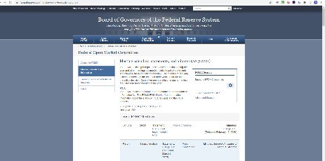
I sourced minutes of FOMC meetings from October 2007 to July 2020 for this analysis (a period for which HTML formatting applies). This gives us a good sample — from the aftermath of the 2007 financial crisis to the period following the 2020 COVID-19 pandemic.
I set up variables for the first part of the URL path (URLPath) and the URL extension (URLExt), as these are common elements of the URL path for all the minutes’ transcripts. I then create a list of dates for the minutes being analyzed (MinutesList).
# Define URLs for the specific FOMC minutes
URLPath = r'https://www.federalreserve.gov/monetarypolicy/fomcminutes'
URLExt = r'.htm'

# List for FOMC minutes from 2007 onward
MinutesList = ['20071031', '20071211', # 2007 FOMC minutes (part-year on new URL format)
           '20080130', '20080318', '20080430', '20080625', '20080805', '20080916', '20081029', '20081216', # 2008 FOMC minutes
           '20090128', '20090318', '20090429', '20090624', '20090812', '20090923', '20091104', '20091216', # 2009 FOMC minutes
           '20100127', '20100316', '20100428', '20100623', '20100810', '20100921', '20101103', '20101214', # 2010 FOMC minutes
           '20110126', '20110315', '20110427', '20110622', '20110809', '20110921', '20111102', '20111213', # 2011 FOMC minutes
           '20120125', '20120313', '20120425', '20120620', '20120801', '20120913', '20121024', '20121212', # 2012 FOMC minutes
           '20130130', '20133020', '20130501', '20130619', '20130731', '20130918', '20131030', '20131218', # 2013 FOMC minutes
           '20140129', '20140319', '20140430', '20140618', '20140730', '20140917', '20141029', '20141217', # 2014 FOMC minutes
           '20150128', '20150318', '20150429', '20150617', '20150729', '20150917', '20151028', '20151216', # 2015 FOMC minutes
           '20160127', '20160316', '20160427', '20160615', '20160727', '20160921', '20161102', '20161214', # 2016 FOMC minutes
           '20172001', '20170315', '20170503', '20170614', '20170726', '20170920', '20171101', '20171213', # 2017 FOMC minutes
           '20180131', '20180321', '20180502', '20180613', '20180801', '20180926', '20181108', '20181219', # 2018 FOMC minutes
           '20190130', '20190320', '20190501', '20190619', '20190731', '20190918', '20191030', '20191211', # 2019 FOMC minutes
           '20200129', '20200315', '20200429', '20200610', '20200729'] # 2020 FOMC minutes
Setting up the corpus
The corpus is the collection of FOMC meeting transcripts that we’re analyzing. It’s also what we use to train our LDA model.
There are several steps in setting up the corpus:
- Text pre-processing — clean the transcripts by removing special characters, extra spaces, stop words and punctuation, then lemmatizing and selecting the parts-of-speech that we wish to retain (nouns, adjectives and verbs) (see this description to learn more about text pre-processing in natural language workflows)
- Extract paragraphs from each of the transcripts — analyzing by paragraph is better for LDA analysis, but we ignore small paragraphs as they don’t add much value (I use a variable called
minparalengthto set the minimum length of paragraph extracted) - Set up lists — containing (i) the paragraphs from all the FOMC minutes (
FOMCMinutes) as a ‘list of lists’, where each sub-list is a paragraph — this is a format suitable for input into the LDA model, (ii) a single list of all the paragraphs (FOMCWordCloud), ie. not a ‘list of lists’, which is used for generating a word cloud of the corpus, and (iii) a list containing the date and ‘weight’ of each paragraph in the corpus (FOMCTopix) — this is needed to aggregate the topic mixes of each paragraph into a combined topic mix for each meeting (see later).
To calculate the weight of each paragraph, first, calculate the total number of characters in each minutes transcript and store this in a variable called cum_paras. Then, for each paragraph, calculate the paragraph’s length (number of characters len(para)) and divide it by cum_paras to arrive at the weight for that paragraph in the minutes transcript. I store the result in FOMCTopix.
Note that the total weights of all paragraphs in a given minutes transcript will sum to 1.
To set up the corpus, I define a function called PrepareCorpus which steps through each of the minutes transcripts, sources it and applies the above steps.
FOMCMinutes = [] # A list of lists to form the corpus
FOMCWordCloud = [] # Single list version of the corpus for WordCloud
FOMCTopix = [] # List to store minutes ID (date) and weight of each para

# Define function to prepare corpus
def PrepareCorpus(urlpath, urlext, minslist, minparalength):

    fomcmins = []
    fomcwordcloud = []
    fomctopix = []

    for minutes in minslist:

        response = requests.get(urlpath + minutes + urlext) # Get the URL response
        soup = BeautifulSoup(response.content, 'lxml') # Parse the response

        # Extract minutes content and convert to string
        minsTxt = str(soup.find("div", {"id": "content"})) # Contained within the 'div' tag

        # Clean text - stage 1
        minsTxt = minsTxt.strip()  # Remove white space at the beginning and end
        minsTxt = minsTxt.replace('\r', '') # Replace the \r with null
        minsTxt = minsTxt.replace(' ', ' ') # Replace " " with space.
        minsTxt = minsTxt.replace(' ', ' ') # Replace " " with space.
        while '  ' in minsTxt:
            minsTxt = minsTxt.replace('  ', ' ') # Remove extra spaces

        # Clean text - stage 2, using regex (as SpaCy incorrectly parses certain HTML tags)
        minsTxt = re.sub(r'(<[^>]*>)|' # Remove content within HTML tags
                         '([_]+)|' # Remove series of underscores
                         '(http[^\s]+)|' # Remove website addresses
                         '((a|p)\.m\.)', # Remove "a.m" and "p.m."
                         '', minsTxt) # Replace with null

        # Find length of minutes document for calculating paragraph weights
        minsTxtParas = minsTxt.split('\n') # List of paras in minsTxt, where minsTxt is split based on new line characters
        cum_paras = 0 # Set up variable for cumulative word-count in all paras for a given minutes transcript
        for para in minsTxtParas:
            if len(para)>minparalength: # Only including paragraphs larger than 'minparalength'
                cum_paras += len(para)

        # Extract paragraphs
        for para in minsTxtParas:
            if len(para)>minparalength: # Only extract paragraphs larger than 'minparalength'

                topixTmp = [] # Temporary list to store minutes date & para weight tuple
                topixTmp.append(minutes) # First element of tuple (minutes date)
                topixTmp.append(len(para)/cum_paras) # Second element of tuple (para weight), NB. Calculating weights based on pre-SpaCy-parsed text

                # Parse cleaned para with SpaCy
                minsPara = nlp(para)

                minsTmp = [] # Temporary list to store individual tokens

                # Further cleaning and selection of text characteristics
                for token in minsPara:
                    if token.is_stop == False and token.is_punct == False and (token.pos_ == "NOUN" or token.pos_ == "ADJ" or token.pos_ =="VERB"): # Retain words that are not a stop word nor punctuation, and only if a Noun, Adjective or Verb
                        minsTmp.append(token.lemma_.lower()) # Convert to lower case and retain the lemmatized version of the word (this is a string object)
                        fomcwordcloud.append(token.lemma_.lower()) # Add word to WordCloud list
                fomcmins.append(minsTmp) # Add para to corpus 'list of lists'
                fomctopix.append(topixTmp) # Add minutes date & para weight tuple to list for storing

    return fomcmins, fomcwordcloud, fomctopix
Now, call the above function to prepare our corpus.
# Prepare corpus
FOMCMinutes, FOMCWordCloud, FOMCTopix = PrepareCorpus(urlpath=URLPath, urlext=URLExt, minslist=MinutesList, minparalength=200)
I set minparalength to 200 — this seems to be a good length for capturing paragraphs which have meaningful content. Shorter paragraphs tend to contain greetings or administrative comments.
Inspecting the corpus
We can see what the prepared corpus looks like by generating a word cloud.
# Generate and plot WordCloud for full corpus
wordcloud = WordCloud(background_color="white").generate(','.join(FOMCWordCloud)) # NB. 'join' method used to convert the documents list to text format
plt.imshow(wordcloud, interpolation='bilinear')
plt.axis("off")
plt.show()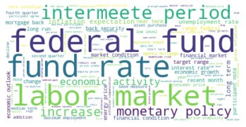
A number of words in the corpus are typical of FOMC meetings, including “federal”, “fund rate”, “market” and “monetary policy”.
Training the LDA model
To train our LDA model, we first need to form a dictionary from our corpus. Map the corpus to word IDs, then convert the words using a bag-of-words approach, and finally apply TF-IDF to the result. This process is called text representation.
# Form dictionary by mapping word IDs to words
ID2word = corpora.Dictionary(FOMCMinutes)

# Set up Bag of Words and TFIDF
corpus = [ID2word.doc2bow(doc) for doc in FOMCMinutes] # Apply Bag of Words to all documents in corpus
TFIDF = models.TfidfModel(corpus) # Fit TF-IDF model
trans_TFIDF = TFIDF[corpus] # Apply TF-IDF model
We use TF-IDF as it produces better results than using bag-of-words alone. TF-IDF adjusts for words that appear frequently but have low semantic value, relative to words that appear infrequently but with higher semantic value. This favors words that have more meaning in the context of the corpus.
For more information about bag-of-words, TF-IDF, and other text representations, see this description.
Next, select the model parameters that we wish to use and run the model.
SEED = 130 # Set random seed
NUM_topics = 8 # Set number of topics
ALPHA = 0.15 # Set alpha
ETA = 1.25 # Set eta

# Train LDA model using the corpus
lda_model = gensim.models.LdaMulticore(corpus=trans_TFIDF, num_topics=NUM_topics, id2word=ID2word, random_state=SEED, alpha=ALPHA, eta=ETA, passes=100)
The parameters shown above are key inputs for an LDA model. NUM_topics, in particular, needs to be set by the user. The other parameters (SEED, ALPHA and ETA) help to produce better results with fine-tuning.
To learn more about LDA parameters and the process for fine-tuning them, please see this description of LDA model evaluation.
How do we evaluate the results of our LDA model?
There are quantitative approaches for doing this, but when applied to a text corpus it’s helpful to produce results that have a sensible human interpretation. This requires judgment.
In terms of quantitative measures, a common measure for evaluating LDA models is the coherence score. This measures the semantic similarity (i.e., the likeness of meaning) between the words in each topic of an LDA model. All else equal, a higher coherence score is better.
We can measure the coherence of our model using the CoherenceModel in gensim.
# Set up coherence model
coherence_model_lda = gensim.models.CoherenceModel(model=lda_model, texts=FOMCMinutes, dictionary=ID2word, coherence='c_v')

# Calculate coherence
coherence_lda = coherence_model_lda.get_coherence()
The coherence score for our model is:
Coherence Score: 0.63779581
This is a fairly good result, based on careful selection of the above parameters.
How did we arrive at our parameters?
In choosing the number of topics (NUM_topics), I was guided by Jegadeesh and Wu, who chose 8 topics for their LDA model — I chose the same, as it tended to produce sensible topic interpretations.
To select the other parameters, you can explore the effect of changing parameter values on model coherence— refer to the section TEST COHERENCE BY VARYING KEY PARAMETERS in the full code listing.
A test of coherence by varying alpha, for instance, results in the following plot (refer to full code listing):
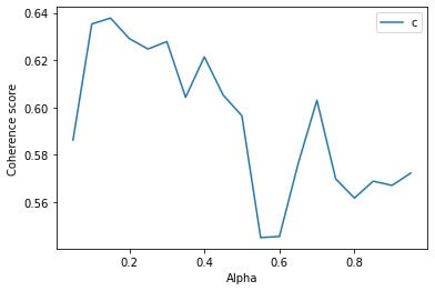
The above plot suggests that an alpha of 0.15 produces a high coherence — this is the value of alpha adopted.
Note that by setting the SEED parameter, we ensure that the model will produce the same results with repeated runs.
Analyzing the topic mix
Since we’re using the same corpus for training and analysis, we don’t need to run the trained LDA model on a new set of documents. Instead, we can go straight to analyzing the corpus.
Our goal is to calculate the topic mix for each of the minutes transcripts in the corpus. By plotting the topic mix over the chronological sequence of the meetings (since each meeting occurred on a given date), we can observe any trends or changes in the topic mix over time.
Recall that we divided our corpus into individual paragraphs, hence our model will produce a topic mix for each paragraph of each transcript in the corpus. The topic mix is a proportionate allocation to each of the (NUM_topics) topics in the model for each paragraph. The proportions across all topics in the paragraph will sum to 1.
We now need to convert these paragraph-level topic mixes to document-level topic mixes (ie. to create an aggregate topic mix for each meeting).
Once again I was guided by Jegadeesh and Wu. They calculate document-level topic mixes (each document being a minutes transcript in our case) using a weighted sum of paragraph-level topic mixes — I adopt the same approach.
We’ve already calculated each paragraph’s weight when we set up our corpus and stored it in FOMCTopix. Let’s call these weights the ‘document-weight’ of each paragraph. Using this, we generate aggregate topic mixes as follows:
- Extract the topic mix for each paragraph and store the result in
FOMCTopixalongside the paragraph’s meeting date and its document-weight - Multiply each topic proportion in the paragraph’s topic mix by the paragraph’s document-weight
- For each document (ie. individual meeting transcript), sum the topic proportions, topic by topic, across all topics for all paragraphs in the transcript
We end up with the weighted topic mixes for each minutes transcript, where the weights are based on the relative lengths of the paragraphs within each transcript.
Extract each paragraph’s topic mix using the get_document_topics method of gensim and append the results to FOMCTopix, which is in a list format. Then, convert this list to a data frame object and call the pivot_table method to sum the topic proportions across all paragraphs within each minutes transcript.
para_no = 0 # Set document counter
for para in FOMCTopix:
    TFIDF_para = TFIDF[corpus[para_no]] # Apply TFIDF model to individual minutes documents
    # Generate and store weighted topic proportions for each para
    for topic_weight in lda_model.get_document_topics(TFIDF_para): # List of tuples ("topic number", "topic proportion") for each para, where 'topic_weight' is the (iterating) tuple
        FOMCTopix[para_no].append(FOMCTopix[para_no][1]*topic_weight[1]) # Weights are the second element of the pre-appended list, topic proportions are the second element of each tuple
    para_no += 1

# Form dataframe of weighted topic proportions (paragraphs) - include any chosen topic names
FOMCTopixDF = pd.DataFrame(FOMCTopix, columns=['Date', 'Weight', 'Inflation', 'Topic 2', 'Consumption', 'Topic 4', 'Market', 'Topic 6', 'Topic 7', 'Policy'])

# Aggregate topic mix by minutes documents (weighted sum of paragraphs)
TopixAggDF = pd.pivot_table(FOMCTopixDF, values=['Inflation', 'Topic 2', 'Consumption', 'Topic 4', 'Market', 'Topic 6', 'Topic 7', 'Policy'], index='Date', aggfunc=np.sum)
Note that I have assigned names to some of the topics in the above code — I’ll discuss this in the next section.
Interpreting topics
Although LDA topic modeling is a quantitative process, the identified topics may not always lend themselves to easy interpretation. You can apply judgment in how you label and select topics depending on your analysis.
You can explore topic contents by generating word clouds.
topic = 0 # Initialize counter
while topic < NUM_topics:
    # Get topics and frequencies and store in a dictionary structure
    topic_words_freq = dict(lda_model.show_topic(topic, topn=50)) # NB. the 'dict()' constructor builds dictionaries from sequences (lists) of key-value pairs - this is needed as input for the 'generate_from_frequencies' word cloud function
    topic += 1

    # Generate Word Cloud for topic using frequencies
    wordcloud = WordCloud(background_color="white").generate_from_frequencies(topic_words_freq)
    plt.imshow(wordcloud, interpolation='bilinear')
    plt.axis("off")
    plt.show()
In our case, I had set 8 topics in the modeling (NUM_topics = 8) based on guidance from Jegadeesh and Wu [1]. This resulted in topics that had a high coherence and good interpretability. Not all of the 8 topics were entirely useful however — some of them were a bit ‘noisy’ and didn’t add much to the analysis. I therefore chose 4 topics on which to focus.
Saret and Mitra also used 8 topics in their modeling but reconfigured this into a smaller number of topics (6 in their analysis), based on what they considered to be sensible interpretations.
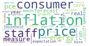
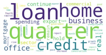
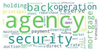
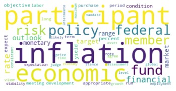
For the 4 topics which I chose, I assigned labels based on the words in the topics and also in comparison with labels used by Jegadeesh and Wu. The topics and labels that I chose are:
- Inflation
- Consumption
- Market
- Policy
The word clouds for these topics are shown below.
Topic mix results
We’re now ready to plot the topic mix of our chosen topics over time.
# Plot results - select which topics to print
TopixAggDF.plot(y=['Inflation', 'Consumption', 'Market', 'Policy'], kind='line', use_index=True)
Let’s see what this looks like:
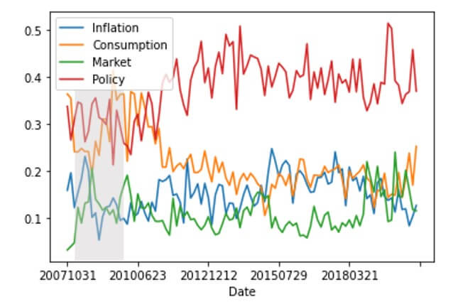
The shaded region (2008–09) represents a US recession period (NBER-designated). The x-axis shows the date of FOMC meetings and the y-axis shows the proportion of each meeting that each topic makes up, based on our analysis.
Interpreting the results
We can observe the following from our plot of the FOMC topic mix over time:
- There’s a noticeable variation in the topic mix over time, particularly for the policy and consumption topics
- There was a significant increase in the time allocated to discussing policy in the period following the 2008–09 recession, and this coincided with a significant reduction in the time spent discussing consumption
- Time spent discussing inflation and the market has been more stable, albeit with a higher proportion during the recession and some divergence during 2014–2018 (ie. more time on inflation and less time on the market)
These observations appear to make sense in light of historical circumstances.
Policy discussions in particular have been an important area for the FOMC since the 2008–09 recession. This reflects the role that monetary policy has had on US financial markets since then, and the significant policy decisions that the FOMC has made (eg. changing the federal funds target rate from over 5% in 2007 to below 0.25% by 2009).
The increase in time spent discussing inflation since 2014 (until recently) reflects the degree of concern the FOMC has had around the management of inflation (which has been persistently low).
Similarly, it’s not surprising that more time than usual has been spent discussing financial markets during the recession and also more recently (starting from a low level prior to 2007). There were important market operations that were initiated or amended during these times.
While subject to some judgment and interpretation, the LDA model has provided a useful quantitative synopsis of the FOMC topic mix over time. This illustrates the potential for NLP techniques to assist the money management process.
In the words of Saret and Mitra:
“Market observers trying to glean insights from [FOMC] meeting minutes once needed to rely on the subjective interpretation of so-called expert “Fed watchers” or their own interpretation. Now, asset allocators can apply natural language processing techniques to extract insights from the FOMC’s published meeting minutes, turning qualitative inputs into more easily analyzed, quantitative data.”
J. N. Saret and S. Mitra, An AI Approach to Fed Watching (2016), Two Sigma Street View, pp. 3-4
Conclusion
Topic modeling is a versatile and evolving area of natural language processing. In this article, we’ve seen how topic modeling can be used to observe the changing mix of topics in a text corpus over time.
Such use cases have the potential for a range of real-world applications. In relation to money management, topic modeling is already being added to the toolkit for making sense of financial markets (as evidenced by Saret and Mitra).