Can BERT Understand Fedspeak?

Natural language processing (NLP) has made great strides in recent years. A notable advance in this area is BERT, a pre-trained language model released by Google in 2018. With BERT, text data can be analyzed to state-of-the-art results with relative ease. But how well does BERT understand ‘fedspeak’, the notoriously vague language used by central bankers? In this article, we explore BERT and fedspeak.

---

Contents

• What is fedspeak?
• NLP and BERT
• What are BERT embeddings?
• The structure of BERT embeddings
• Applying BERT to fedspeak
• Implementation in Python
  • The full code
  • Stepping through the code
    • Import libraries
    • Source FOMC minutes
    • Text pre-processing (step 1 of the NLP workflow)
    • BERT embeddings (step 2 of the NLP workflow)
    • Visualize embeddings
    • Calculate similarity between embeddings
    • Generate similarity matrix
• Conclusion

In this article, we apply BERT to fedspeak by analyzing a Federal Open Market Committee (FOMC) transcript.

We investigate how well BERT differentiates sentences in the transcript by calculating the similarity between sentence embeddings.

If we find that similarity scores between embeddings look sensible, based on our own (human) interpretation, then this suggests that BERT is doing a good job at understanding fedspeak.

What is fedspeak?

Fedspeak refers to the language used by central bankers.

It was originally coined to describe how Alan Greenspan spoke about the economy and financial markets.

Greenspan was chair of the US Federal Reserve from 1987 to 2006 and was notorious for using vague and unclear language—he’s been described as “a master of the strategic mumble“¹ for this reason.

Greenspan’s words could significantly move financial markets. This is why he preferred to use vague language—he didn’t want to give away too much about what the central bank was thinking.

Fedspeak continues to be used by central bankers today, and in particular during FOMC meetings. These meetings are a forum for discussing the state of the US economy and associated policies.

FOMC meetings take place eight times per year and the minutes from these meetings contain a wealth of information for investors—provided they can understand fedspeak!

NLP and BERT

With recent advances in natural language processing (NLP), all manner of text analyses are now possible. NLP can assist with customer service, language translation, speech recognition, sentiment analysis, and document classification amongst other tasks.

What’s more, with today’s computing power and cutting-edge algorithms, NLP can achieve a speed and accuracy that’s far beyond what was possible only a few years ago.

But, can NLP understand fedspeak?

In this article, we explore the application of NLP to fedspeak using a powerful tool called BERT.

BERT, or Bidirectional Encoder Representations from Transformers, is a language model developed by Google and released in 2018.

BERT provides free access to powerful pre-trained language representations. It can extract language features from text data (as we do in this article) or fine-tune models for specific NLP tasks.

BERT makes it easy to achieve state-of-the-art NLP results without a massive training effort, thanks to its built-in pre-training. BERT’s release was a significant milestone, promoting a new era of NLP deployment.

A particularly useful feature of BERT is its ability to capture the context of word representations. This sets it apart from predecessors like word2vec or GloVe.

Being able to differentiate words based on their context, such as ‘bank’ in ‘bank account’ vs ‘river bank’, leads to more effective NLP models.

What are BERT embeddings?

BERT embeddings are individual number vectors that represent each word (or combinations of words) in a text document.

NLP works by converting text into a set of numbers for further analysis. This process is referred to as the NLP workflow and has three key steps: text pre-processing, text representation, and analysis.

With BERT, the first two steps of the NLP workflow result in BERT embeddings.

The structure of BERT embeddings

Each BERT embedding (based on the version we use in this article) has 768 dimensions. These dimensions are also called hidden units or features and they represent a set of unique characteristics for each word.

Each word can be mapped to a multi-dimensional vector space based on the 768 dimensions, and the inter-relationships between words can be expressed in terms of the interaction between the vectors.

Each BERT embedding also has a number of layers—1 input layer and 12 output layers—each of which has 768 dimensions. That’s a lot of numbers to represent a single word!

But it’s one of the reasons why BERT is so powerful—the quantum of information dedicated to each word helps to capture a meaningful representation.

BERT gives you a choice about which output layer, or combination of layers, you use for your analysis. The choice depends on the type of analysis that you’re doing, and it’s not always easy to know in advance which layer will work best.

In this article, we use an approach that works well in a range of circumstances, but there are other choices that are possible. More about this later.

Applying BERT to fedspeak

We explore how BERT interprets FOMC fedspeak using the following approach:

• Get the minutes transcript from a recent FOMC meeting—this is the text that we’ll be analyzing
• Prepare and pre-process the text, then separate it into sentences
• Convert the words in each sentence into BERT embeddings, then aggregate these to form sentence embeddings
• Look at the similarity between sentence embeddings (using cosine similarity) and see how it compares with human (i.e., our) interpretation

If the similarity measures make sense, i.e., that similar sentences score high, and dissimilar sentences score low, then this is a sign that BERT is successfully interpreting the FOMC minutes. Or in other words, it’s a sign that BERT understands fedspeak.

Implementation in Python

Tthe following sets out the full code and then steps through the key sections of code to explain the analysis.

The code is implemented in Python (v3.8.3).

You can jump straight to the step-through of the code here.

The full code:

 #####################################
 ### APPLYING BERT TO FOMC MINUTES ###
 #####################################
  
 ### Import libraries ###
  
 import requests
 import re
 from bs4 import BeautifulSoup
 import pandas as pd
 import numpy as np
 import matplotlib.pyplot as plt
  
 import spacy
 nlp = spacy.load("en_core_web_lg")
 nlp.max_length = 1500000 # In case max_length is set to lower than this (ensure sufficient memory)
  
 import umap # Dimensionality reduction
 from scipy.spatial.distance import cosine # For calculating cosine distance
  
 # Using BERT with PyTorch
 import torch
 from transformers import BertTokenizer, BertModel
 tokenizer = BertTokenizer.from_pretrained('bert-base-uncased')
  
 ### GRAB THE DOCUMENT BY PARSING URL ###
  
 # Define URL for the specific FOMC minutes
 URLPath = r'https://www.federalreserve.gov/monetarypolicy/fomcminutes' # Relevant for FOMC minutes from 2008 onward
 URLExt = r'.htm'
  
 # Date of FOMC meeting transcript being analyzed
 Minutes = '20200729'
  
 ### SET UP THE TRANSCRIPT FOR ANALYSIS ###
  
 FOMCMinutes = [] # List of sentence tokens
  
 # Define function to pre-process text (parsing FOMC minutes and tokenizing sentences)
 def TextPreProcess(urlpath, urlext, minutes, minsentlength):
     
     # Get meeting minutes from the FOMC website    
     response = requests.get(urlpath + minutes + urlext) # Get the URL response
     soup = BeautifulSoup(response.content, 'lxml') # Parse the response
         
     # Extract minutes content and convert to string
     minsTxt = str(soup.find("div", {"id": "content"})) # Contained within the 'div' tag
                     
     # Clean text - stage 1
     minsTxt = minsTxt.strip()  # Remove white space at the beginning and end
     minsTxt = minsTxt.replace('\r', '') # Replace the \r with null
     minsTxt = minsTxt.replace('\n', ' ') # Replace the \n with space
     minsTxt = minsTxt.replace(' ', ' ') # Replace " " with space. 
     minsTxt = minsTxt.replace(' ', ' ') # Replace " " with space.
     while '  ' in minsTxt:
         minsTxt = minsTxt.replace('  ', '') # Remove extra spaces
  
     # Clean text - stage 2, using regex (as SpaCy incorrectly parses certain HTML tags)    
     minsTxt = re.sub(r'(<[^>]*>)|' # Remove content within HTML tags
                      '([_]+)|' # Remove series of underscores
                      '(http[^\s]+)', # Remove website addresses
                      '', minsTxt) # Replace with null
  
     fomcminsTMP = list(nlp(minsTxt).sents) # List of sentences in minsTxt
  
     # Initialize list of sentnce tokens
     fomcmins = []
  
     # Keep only sentences with more than 'minsentlength' tokens in length but less than 500 tokens (to avoid overflow issues in BERT)
     for sentence in fomcminsTMP:
         if len(sentence) > minsentlength and len(sentence) < 500:
             fomcmins.append(str(sentence)) # Add sentence to sentence tokens list, converting to string
                 
     return fomcmins
  
 # Pre-process text
 FOMCMinutes = TextPreProcess(urlpath=URLPath, urlext=URLExt, minutes=Minutes, minsentlength=10)
  
 ### Create BERT embeddings ###
  
 sentence_embeddings = []
 count = 0
  
 # Total number of sentences
 print("There are " + str(len(FOMCMinutes)) + " sentences in total:")
  
 # Define function for creating BERT sentence embeddings
 for sentence in FOMCMinutes:
     
     marked_text = "[CLS]" + sentence + "[SEP]" # BERT tokenizer requirement
     tokenized_text = tokenizer.tokenize(marked_text) # Use BERT to tokenize
     indexed_tokens = tokenizer.convert_tokens_to_ids(tokenized_text) # Map tokens to BERT's vocabulary indices
     segments_ids = [1] * len(tokenized_text) # BERT requires IDs for each token - an ID of 1 is sufficient since working with one sentence at a time
     
     # Convert inputs to tensors (using PyTorch) - required for calling the BERT model
     tokens_tensor = torch.tensor([indexed_tokens])
     segments_tensors = torch.tensor([segments_ids])
     
     # Load pre-trained model (weights)
     model = BertModel.from_pretrained('bert-base-uncased', output_hidden_states = True) # Return all hidden-states
                                   
     # Put the model in evaluation mode (feed-forward operation only)
     model.eval()
     
     # Run BERT and collect all of the hidden states produced for all 12 layers
     with torch.no_grad(): # 'no_grad' tells PyTorch not to construct the compute graph during the forward pass - reduces memory and improves speed
         outputs = model(tokens_tensor, segments_tensors)
         hidden_states = outputs[2] # 3rd item returns hidden states from all layers
     
     # Creating sentence vectors by averaging acrross the second-to-last hidden layers of each token
     token_vecs = hidden_states[-2][0] # Accessing the second-to-last hidden layers
     sentence_embed = torch.mean(token_vecs, dim=0) # Calculating average across all tokens
     sentence_embeddings.append(sentence_embed.numpy()) # Convert 'sentence_embed' tensor to numpy array
     
     # Simple progress counter
     count += 1
     if (count % 50) == 0: # Counter by each 100 sentences
         print("At sentence number ..." + str(count))
  
 ### Visualize embeddings in 2D ###
  
 # Reduce dimensionality to 2, for 2D plotting
 umap_embeddings_B = umap.UMAP(n_neighbors=15, n_components=2, min_dist=0.0, metric='cosine').fit_transform(sentence_embeddings) # Dimension reduction to 2D
 result = pd.DataFrame(umap_embeddings_B, columns=['x', 'y']) # Store 2D results
  
 # Plot
 fig, ax = plt.subplots()
 plt.scatter(result.x, result.y, s=0.3)#, cmap='magma')
  
 ### Measure similarity between sentence embeddings ###
  
 # Generate cosine similarity matrix
 sim_matrix = []
 embeddings_length = len(sentence_embeddings)
  
 for count1 in range(0,embeddings_length):
     inner_matrix = []
     inner_matrix_plt = []
     for count2 in range(0,embeddings_length-(embeddings_length-count1)):
         inner_matrix.append(1 - cosine(sentence_embeddings[count1], sentence_embeddings[count2])) # Cosine similarity (values of 0 to 1)
     sim_matrix.append(inner_matrix)
     
 similarity_matrix = pd.DataFrame(sim_matrix)
  
 # Plot cosine similarity matrix
 plt.matshow(similarity_matrix, cmap='viridis')
 plt.colorbar()
 plt.show

Stepping through the code:

Import libraries

First, import libraries to do the following:

• Request and parse the FOMC minutes transcript (requests and BeautifulSoup)
• Pre-process text (regular expressions and spacy)
• Analyze and display results (pandas, numpy and matplotlib)
• Generate BERT embeddings (transformers and torch)
• Reduce dimensionality of the embeddings for plotting in 2D (umap)
• Calculate cosine similarity (scipy)

 ### Import libraries ###
  
 import requests
 import re
 from bs4 import BeautifulSoup
 import pandas as pd
 import numpy as np
 import matplotlib.pyplot as plt
  
 import spacy
 nlp = spacy.load("en_core_web_lg")
 nlp.max_length = 1500000 # In case max_length is set to lower than this (ensure sufficient memory)
  
 import umap # Dimensionality reduction
 from scipy.spatial.distance import cosine # For calculating cosine distance
  
 # Using BERT with PyTorch
 import torch
 from transformers import BertTokenizer, BertModel
 tokenizer = BertTokenizer.from_pretrained('bert-base-uncased') 

Source FOMC minutes

FOMC minutes transcripts are available from the FOMC website.

We’ll analyze the minutes from the meeting FOMC on 29 July 2020.

 ### GRAB THE DOCUMENT BY PARSING URL ###
  
 # Define URL for the specific FOMC minutes
 URLPath = r'https://www.federalreserve.gov/monetarypolicy/fomcminutes' # Relevant for FOMC minutes from 2008 onward
 URLExt = r'.htm'
  
 # Date of FOMC meeting transcript being analyzed
 Minutes = '20200729' 

Text pre-processing (step 1 of the NLP workflow)

In the first part of the NLP workflow, prepare the transcript as follows:

• Get the URL response and parse the text using requests and BeautifulSoup
• Clean the text in a two-stage process, first using search-and-replace and second using regular expressions
• Separate the text into sentences using spacy
• Check the word length of each sentence
• Form a list of sentences that meet the word-length criteria

Only include sentences that are long enough to have a purposeful meaning but not so long as to cause an issue for the BERT algorithm. Use sentences of between 10 and 500 words for this purpose—this will be our word-length criteria.

With this approach, we end up with 310 individual sentences in our transcript.

 ### SET UP THE TRANSCRIPT FOR ANALYSIS ###
  
 FOMCMinutes = [] # List of sentence tokens
  
 # Define function to pre-process text (parsing FOMC minutes and tokenizing sentences)
 def TextPreProcess(urlpath, urlext, minutes, minsentlength):
     
     # Get meeting minutes from the FOMC website    
     response = requests.get(urlpath + minutes + urlext) # Get the URL response
     soup = BeautifulSoup(response.content, 'lxml') # Parse the response
         
     # Extract minutes content and convert to string
     minsTxt = str(soup.find("div", {"id": "content"})) # Contained within the 'div' tag
                     
     # Clean text - stage 1
     minsTxt = minsTxt.strip()  # Remove white space at the beginning and end
     minsTxt = minsTxt.replace('\r', '') # Replace the \r with null
     minsTxt = minsTxt.replace('\n', ' ') # Replace the \n with space
     minsTxt = minsTxt.replace(' ', ' ') # Replace " " with space. 
     minsTxt = minsTxt.replace(' ', ' ') # Replace " " with space.
     while '  ' in minsTxt:
         minsTxt = minsTxt.replace('  ', '') # Remove extra spaces
  
     # Clean text - stage 2, using regex (as SpaCy incorrectly parses certain HTML tags)    
     minsTxt = re.sub(r'(<[^>]*>)|' # Remove content within HTML tags
                      '([_]+)|' # Remove series of underscores
                      '(http[^\s]+)', # Remove website addresses
                      '', minsTxt) # Replace with null
  
     fomcminsTMP = list(nlp(minsTxt).sents) # List of sentences in minsTxt
  
     # Initialize list of sentnce tokens
     fomcmins = []
  
     # Keep only sentences with more than 'minsentlength' tokens in length but less than 500 tokens (to avoid overflow issues in BERT)
     for sentence in fomcminsTMP:
         if len(sentence) > minsentlength and len(sentence) < 500:
             fomcmins.append(str(sentence)) # Add sentence to sentence tokens list, converting to string
                 
     return fomcmins
  
 # Pre-process text
 FOMCMinutes = TextPreProcess(urlpath=URLPath, urlext=URLExt, minutes=Minutes, minsentlength=10)

BERT embeddings (step 2 of the NLP workflow)

After pre-processing the text, the second part of the NLP workflow converts it to vectors (BERT embeddings). We’re guided by the insightful tutorial on this topic by Chris McCormick and Nick Ryan².

Note that the approach used in this article is a little more hands-on than necessary. This gives us a better understanding of what’s happening. As Chris McCormick points out, there are tensorflow and pytorch implementations that provide more direct approaches for BERT embeddings.

We use the pytorch interface for BERT, developed by Hugging Face, to generate our embeddings. This is a versatile package offering a useful level of detail while remaining easy to use.

You’ll need to install the Hugging Face package before using it for the first time (you can find information on how to do it here).

Do the following for each sentence of the pre-processed text:

• Tokenize each word in the sentence
• Add special tokens and IDs according to BERT algorithm requirements
• Convert the tokenized words into tensors
• Run the BERT algorithm to generate word embeddings
• Extract the relevant layer from each word embedding and aggregate it across all words in the sentence to form a sentence embedding
• Go to the next sentence and repeat

Recall that BERT embeddings have 12 output layers to choose from. We’ll choose the second-to-last output layer, which is the approach used by Han Xiao, creator of the bert-as-service GitHub project.

Xiao’s rationale for using the second-to-last layer is (as summarized by Chris McCormick):

• The first output layer of a BERT embedding does not contain much contextual information
• As you move through the output layers, contextual information increases
• At the final layer, information that is specific to certain pre-training tasks starts to become more dominant, which may not be relevant for your own analysis
• The second-to-last layer is a sweet spot, ie. a good balance between contextual information and task-specific information

Now that we know which embedding layer to use, how do we form sentence embeddings from word embeddings?

Again, there are different ways to do this.

Chris McCormick suggests a simple approach of averaging across all words in a sentence to produce a sentence embedding. We use this approach, and in our case, this means averaging the second-to-last output layer of each word embedding to produce the sentence embedding.

 ### Create BERT embeddings ###
  
 sentence_embeddings = []
 count = 0
  
 # Total number of sentences
 print("There are " + str(len(FOMCMinutes)) + " sentences in total:")
  
 # Define function for creating BERT sentence embeddings
 for sentence in FOMCMinutes:
     
     marked_text = "[CLS]" + sentence + "[SEP]" # BERT tokenizer requirement
     tokenized_text = tokenizer.tokenize(marked_text) # Use BERT to tokenize
     indexed_tokens = tokenizer.convert_tokens_to_ids(tokenized_text) # Map tokens to BERT's vocabulary indices
     segments_ids = [1] * len(tokenized_text) # BERT requires IDs for each token - an ID of 1 is sufficient since working with one sentence at a time
     
     # Convert inputs to tensors (using PyTorch) - required for calling the BERT model
     tokens_tensor = torch.tensor([indexed_tokens])
     segments_tensors = torch.tensor([segments_ids])
     
     # Load pre-trained model (weights)
     model = BertModel.from_pretrained('bert-base-uncased', output_hidden_states = True) # Return all hidden-states
                                   
     # Put the model in evaluation mode (feed-forward operation only)
     model.eval()
     
     # Run BERT and collect all of the hidden states produced for all 12 layers
     with torch.no_grad(): # 'no_grad' tells PyTorch not to construct the compute graph during the forward pass - reduces memory and improves speed
         outputs = model(tokens_tensor, segments_tensors)
         hidden_states = outputs[2] # 3rd item returns hidden states from all layers
     
     # Creating sentence vectors by averaging acrross the second-to-last hidden layers of each token
     token_vecs = hidden_states[-2][0] # Accessing the second-to-last hidden layers
     sentence_embed = torch.mean(token_vecs, dim=0) # Calculating average across all tokens
     sentence_embeddings.append(sentence_embed.numpy()) # Convert 'sentence_embed' tensor to numpy array
     
     # Simple progress counter
     count += 1
     if (count % 50) == 0: # Counter by each 100 sentences
         print("At sentence number ..." + str(count))

Visualize embeddings

Recall that there are 768 dimensions in each embedding—how can we visualize this?

We need to first reduce the dimensions of our sentence embeddings to visualize them. We use umap to do this, following Maarten Grootendorst‘s suggestion in his excellent article, reducing our embeddings from 768 dimensions to two dimensions (2D).

Once we’ve reduced the dimensions of our sentence embeddings, we can plot the results.

 ### Visualize embeddings in 2D ###
  
 # Reduce dimensionality to 2, for 2D plotting
 umap_embeddings_B = umap.UMAP(n_neighbors=15, n_components=2, min_dist=0.0, metric='cosine').fit_transform(sentence_embeddings) # Dimension reduction to 2D
 result = pd.DataFrame(umap_embeddings_B, columns=['x', 'y']) # Store 2D results
  
 # Plot
 fig, ax = plt.subplots()
 plt.scatter(result.x, result.y, s=0.3)

Here’s what the embeddings look like in 2D:

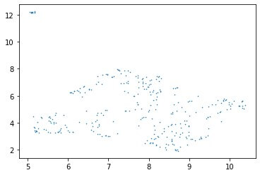
Most of the embeddings are clustered in a broad area towards the bottom of the plot, with a handful in the top-left.

Note that the umap algorithm is stochastic, which means the results will vary with each run. Hence, the 2D plot will also vary with each run. This won’t change the underlying multi-dimensional BERT embeddings, however.

Embeddings that are closer together in the plot represent sentences that are more similar to each other, while embeddings that are far from each other represent sentences that are more different. Let’s explore this by calculating the similarity between embeddings.

Calculate similarity between embeddings

We can use cosine similarity to calculate the similarity between embeddings.

Cosine similarity measures the cosine of the angle between two vectors in multi-dimensional space.

In our case, the two vectors are the multi-dimensional sentence embeddings, with 768 dimensions each.

Cosine similarity is a popular measure that’s often used for comparing text documents. It produces values in a range from 0 to 1.

A value closer to 0 implies less similarity and a value closer to 1 implies more similarity.

Let’s look at a few examples of similarity between our embeddings.

We can use the cosine function from the scipy package to calculate the similarity between any two vectors as follows: cosine similarity = 1 - cosine(vector 1, vector 2)

Consider the following two sentences in our FOMC minutes transcript. They have a cosine similarity score of nearly 1:

This assessment would take into account a wide range of information, including measures of labor market conditions, indicators of inflation pressures and inflation expectations, and readings on financial and international developments.

Sentence 1

This assessment will take into account a wide range of information, including measures of labor market conditions, indicators of inflation pressures and inflation expectations, and readings on financial and international developments.

Sentence 2

Sentences 1 and 2 are nearly identical, hence a similarity score of close to 1 makes sense.

Let’s consider another pair of sentences that are also similar but less identical:

Deputy Associate Directors, Division of Monetary Affairs, Board of Governors; Luca Guerrieri, Deputy Associate Director, Division of Financial Stability, Board of Governors; Norman J. Morin, Deputy Associate Director, Division of Research and Statistics, Board of Governors; Jeffrey D. Walker

Sentence 3

Deputy Associate Director, Division of Reserve Bank Operations and Payment Systems, Board of Governors Brian J. Bonis and Etienne Gagnon,3 Assistant Directors, Division of Monetary Affairs, Board of Governors; Viktors Stebunovs,5 Assistant Director, Division of International Finance, Board of Governors Brett Berger,6 Adviser, Division of International Finance, Board of Governors

Sentence 4

The similarity score between sentences 3 and 4 is very high, around 0.96. Does this make sense?

Sentences 3 and 4 are similar in that they both appear to perform a similar function—listing out the names and positions of various FOMC stakeholders. A high similarity score makes sense.

Now, let’s consider sentences that have a low similarity score:

Jerome H. Powell, Chair John C. Williams, Vice Chair

Sentence 5

Following sharp declines, economic activity and employment have picked up somewhat in recent months but remain well below their levels at the beginning of the year.

Sentence 6

Sentences 5 and 6 have a similarity score of 0.39, one of the lowest amongst our embeddings.

The sentences are clearly quite different in their content and their intent. It makes sense that they have a low similarity score.

Another example of sentences that have a low similarity score is as follows:

Altogether, the available data suggested that net exports were a significant drag on the rate of change in real GDP in the second quarter.

Sentence 7

The meeting adjourned at 10:55 a.m. on July 29, 2020.

Sentence 8

Sentences 7 and 8 are clearly different. One discusses economic data and the other is an administrative note.

Here, too, a low similarity score makes sense.

Generate similarity matrix

Now, let’s look at the cosine similarity between all of the sentence embeddings in our transcript.

Recall that there are 310 sentences and hence 310 sentence embeddings in our analysis.

To calculate the cosine similarity between all of our sentences, we would need to compare each sentence embedding with each other, implying 310 x 310 calculations. That’s over 96,000 calculations in total!

But, we can simplify this by noting that half of the calculations are redundant.

Cosine similarity is a symmetric measure, so the similarity between variable 1 and variable 2 is the same as the similarity between variable 2 and variable 1. Hence, half of the calculations would be identical to the other half and would not need to be calculated twice.

In addition, the similarity between the same sentences (i.e., a sentence’s similarity with itself) will have a value of 1 and does not need to be calculated. These would form the diagonal of the matrix.

So, we only need to calculate half of the similarities, producing a half-filled matrix of values.

This will look like a triangle of values, much the same as if we were calculating a correlation or covariance matrix.

We can generate a similarity matrix as follows:

 ### Measure similarity between sentence embeddings ###
  
 # Generate cosine similarity matrix
 sim_matrix = []
 embeddings_length = len(sentence_embeddings)
  
 for count1 in range(0,embeddings_length):
     inner_matrix = []
     inner_matrix_plt = []
     for count2 in range(0,embeddings_length-(embeddings_length-count1)):
         inner_matrix.append(1 - cosine(sentence_embeddings[count1], sentence_embeddings[count2])) # Cosine similarity (values of 0 to 1)
     sim_matrix.append(inner_matrix)
     
 similarity_matrix = pd.DataFrame(sim_matrix)
  
 # Plot cosine similarity matrix
 plt.matshow(similarity_matrix, cmap='viridis')
 plt.colorbar()
 plt.show

Here’s a plot of the similarity matrix:

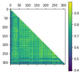
The plot color-codes regions of different similarity with different colors.

Embeddings with a high similarity are more towards the yellow end of the color spectrum, and embeddings with a low similarity are more towards the blue end.

In the sentence examples that we looked at, sentences 1 to 4 (high similarity) would appear close to yellow in color, and sentences 5 to 8 (low similarity) would appear close to blue.

The plot suggests that there is variation in similarity between sentence embeddings, with plenty of yellow (high similarity) interspersed with areas of blue (low similarity).

This differentiation suggests that BERT is functioning well in its efforts to interpret fedspeak.

And as we’ve seen, the similarity metrics based on the BERT embeddings appear to make sense.

Conclusion

NLP is fast-evolving with recent advances that have vastly improved its versatility and scope.

BERT is an example of an NLP model that brings powerful capabilities to the analysis of natural language and text.

In this article, we’ve applied BERT to ‘fedspeak’—the notoriously difficult-to-understand language used by central bankers.

Using BERT, we created sentence embeddings for the transcript of a recent FOMC meeting.

The embeddings transformed the sentences in the transcript into multi-dimensional vectors of numbers. These vectors can be analyzed in various ways.

Based on the embeddings, we explored the similarity between sentences in the transcript.

We found that BERT does a good job of distinguishing between similar and dissimilar sentences in a way that makes sense.

It appears that BERT can indeed understand fedspeak!

We’ve only just scratched the surface of BERT’s possibilities, however.

BERT embeddings can be applied to a number of downstream tasks such as classification and summarization. The success with which this can be done will depend on a range of factors including the algorithms used and the sample of text being analyzed.

In my personal experience, it’s challenging to effectively apply such downstream tasks to FOMC transcripts—but this is a topic for future work.

In the meantime, BERT continues to bring powerful capabilities to NLP analysis.

BERT helps to make sense of text data in a manner that can be automated and scaled and does so while capturing context. It even helps to make sense of fedspeak!

References

[1] James Hookway, In The Eternal Quest to Decode Fedspeak, Here Come the Computers, The Wall Street Journal, February 9, 2020. https://www.wsj.com/articles/in-the-eternal-quest-to-decode-fedspeak-here-come-the-computers-11581287394

[2] Chris McCormick and Nick Ryan,  BERT Word Embeddings Tutorial, May 14, 2019. http://www.mccormickml.com