Bayes Theorem: As  Easy as Checking the Weather

Bayes theorem is a widely used statistical technique. Its applications range from clinical trials to email classification, and its concepts underpin a range of broader use-cases. But is it possible to understand Bayes theorem without getting bogged down in detailed math or probability theory? Yes it is — this article shows you how.

Contents

• What’s the weather like?
• Exploring Bayes theorem
• Independence and conditional independence
• Bayes theorem calculator
• Applications of Bayes theorem
• Conclusion
• FAQs

Bayes theorem is named after the English statistician and Presbyterian minister, Thomas Bayes, who formulated the theorem in the mid 1700’s. Unfortunately, Bayes never lived to see his theorem gain prominence as it was published after his death.

Bayes theorem has since grown to become a widely used and important tool in statistics. It underpins a range of applications in science, engineering, the humanities and artificial intelligence.

What’s the weather like?

To understand Bayes theorem, let’s start by considering a simple example.

Say you wanted to head out for the day and are deciding if you should take an umbrella. You look out the window — it’s cloudy.

Will it rain?

To help you decide, you look at some local weather data over the past 100 days. It says:

• It was cloudy on 40 days
• It rained on 30 days
• It was both raining and cloudy on 25 days

What does this tell you?

Based on this data, you can estimate that the probability it will rain is 30% (ie. 30 days out of 100). Similarly, the probability it’s cloudy is 40%, and the probability it’s both raining and cloudy is 25%.

But, you already know it’s cloudy today since you’ve looked out the window. So, what are the chances that it will rain given it’s cloudy today?

Well, of the 40 cloudy days, 25 were raining. You know this because there were only 25 days on which it was both cloudy and raining.

So, the probability that it will rain given it’s cloudy must be 25 days / 40 days = 62.5%.

Let’s now consider a different perspective.

You look out the window and let’s imagine it’s raining but not cloudy (a ‘sun shower’). Will it become cloudy?

We’re now trying to estimate the probability that it will be cloudy given it’s raining.

Again, we know that it was both cloudy and raining on 25 days and also that it was raining on 30 days. Hence, when it’s raining, the probability that it’s also cloudy must be 83.3% (25 days out of 30 days).

So, the the probability that it will be cloudy given it’s raining is 83.3%.

You’ve just calculated a couple of conditional probabilities.

Exploring Bayes theorem

To make things clearer, let’s apply some notation to our example:

Let “the probability that it will be cloudy” be “prob(cloudy)”

Similarly,

• The probability that it will rain is prob(rain)
• The probability that it will be both raining and cloudy is prob(rain & cloudy)
• The probability that it will rain given it’s cloudy is prob(rain|cloudy)
• The probability that it will be cloudy given it’s raining is prob(cloudy|rain)

Conditional probabilities

You’ll notice we’re using the symbol “|” to mean “given”, which is another way of saying “conditional upon”. So, prob(rain|cloudy) and prob(cloudy|rain) are both conditional probabilities.

In contrast, prob(cloudy) and prob(rain) are not conditional on other variables and may be called unconditional probabilities.

From the example we know that:

• prob(cloudy) = 40%
• prob(rain) = 30%
• prob(rain & cloudy) = 25%
• prob(rain|cloudy) = 62.5%
• prob(cloudy|rain) = 83.3%

Recall that we calculated prob(rain|cloudy) = 25 days / 40 days = 62.5%.

Another way of saying this is:

prob(rain|cloudy) = prob(rain & cloudy) / prob(cloudy)

= 25% / 40% = 62.5% Equation 1

Similarly, prob(cloudy|rain) = prob(rain & cloudy) / prob(rain)

= 25% / 30% = 83.3% Equation 2

Congratulations, you’ve just stepped through the essence of Bayes theorem!

Unpacking Bayes theorem

Bayes theorem is another way of calculating a conditional probability.

In our example, looking at Equation 1 and Equation 2, you’ll notice the term ‘prob(rain & cloudy)’ is common to both.

Rearranging:

prob(rain|cloudy) * prob(cloudy) = prob(rain & cloudy) Equation 3

prob(cloudy|rain) * prob(rain) = prob(rain & cloudy) Equation 4

Equating for the common term ‘prob(rain & cloudy)’ in Equation 3 and Equation 4:

prob(rain|cloudy) * prob(cloudy) = prob(cloudy|rain) * prob(rain)

Rearranging:

prob(rain|cloudy) = [prob(cloudy|rain)*prob(rain)] / prob(cloudy)

This is Bayes theorem, applied to our example.

We could also write:

prob(cloudy|rain) = [prob(rain|cloudy)*prob(cloudy)] / prob(rain)

If we were to generalize the expression, we could write:

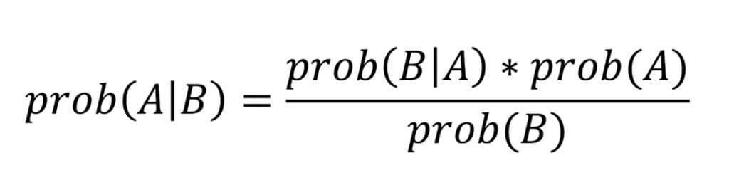
This is Bayes theorem, applied to any ‘events’ A and B.

You may hear the terms posterior probability or prior probability used in relation to Bayes theorem. These refer to ‘prob(A|B)’ and ‘prob(A)’ respectively in our general expression above.

The idea is that the prior probability is an existing estimate and the posterior probability is an updated estimate based on additional information (B).

Is it going to rain?

Let’s now use Bayes theorem to answer our original question, “the probability that it will rain given it’s cloudy?”:

prob(rain|cloudy) = [prob(cloudy|rain) * prob(rain)] / prob(cloudy)

= [83.3% * 30%] / 40%

= 62.5%

So, we’ve used Bayes theorem to calculate our answer, which is a conditional probability, and it agrees with our earlier answer (62.5%).

But, if we can get to our answer directly, why do we need Bayes theorem?

When to use Bayes theorem

Bayes theorem is useful when you don’t have enough information to directly calculate a conditional probability.

In our example, let’s say we say we knew only the following:

• prob(cloudy) = 40%
• prob(rain) = 30%
• prob(cloudy|rain) = 83.3%

If we wanted to estimate prob(rain|cloudy), our original question, we could use Bayes theorem to calculate it (62.5%).

As it happens, probabilities such as prob(rain & cloudy), which are called joint probabilities, are often difficult to calculate. Conditional probabilities, on the other hand, can be easier to calculate and we can use Bayes theorem to calculate one conditional probability from another.

Independence and conditional independence

Another important concept related to conditional probabilities is conditional independence. This can greatly simplify statistical calculations and can be applied to Bayes theorem to produce useful results, as we’ll see later.

For now, let’s take a closer look at independence and conditional independence.

Two variables a and b are said to be independent if:

prob(a and b) = prob(a) * prob(b) Equation 5

When a and b are independent, then:

prob(a|b) = prob(a)

and,

prob(b|a) = prob(b)

Note that you can see this from Bayes theorem. If a and b are independent, then under Bayes theorem:

prob(a|b) = [prob(b|a) * prob(a)] / prob(b)

But, since a and b are independent, prob(b|a) = prob(b). Hence,

prob(a|b) = [prob(b) * prob(a)] / prob(b) = prob(a).

Two variables a and b are said to be conditionally independent with respect to a third variable c if:

prob(a|c) = prob(a|b and c)

Why does all this matter?

Independence makes calculating joint probabilities much easier.

Recall, we said that joint probabilities are difficult to calculate — if the underlying events are independent, then the joint probability is simply the product of the individual probabilities (Equation 5).

But we won’t always know if two events are independent. We may know, however, if two events are independent conditional upon a third event. This results in conditional independence.

To make this clearer, let’s look at some examples from Aerin Kim, a data scientist who has written a more comprehensive, technical description of conditional independence.

Consider the following examples:

1. Lung cancer, yellow teeth | smoking—is there a relationship between lung cancer and yellow teeth for a person, given that the person is a smoker?
2. Car starter motor working, car radio working | battery—is there a relationship between a car starter motor and a car radio, given that both depend on a car battery?
3. Amount of speeding fine, type of car | speed—is there a relationship between speeding fines and the type of car, given the presence of high speed?

Looking at the first example, there’s no particular relationship between lung cancer and yellow teeth, but they may often occur together. In other words, there’s a correlation between the two. This may lead us to believe there is indeed a relationship, or causation between them (ie. we may think they’re not independent).

If we take account of smoking, however, then the apparent relationship disappears — it’s smoking that causes both lung cancer and yellow teeth rather than lung cancer causing yellow teeth (or the other way around). So, lung cancer and yellow teeth are independent conditional on smoking, or in other words they’re conditionally independent.

We can look at the second and third examples in the same way. There’s no direct relationship, for instance, between a car starter motor and a car radio, but both depend on the battery. So, although they may appear to be related, the starter motor and radio are conditionally independent based on the battery. 

These examples of conditional independence highlight another important concept in statistics — correlation vs causation. Just because two events seem correlated, it doesn’t necessarily mean that one causes the other. They may actually be conditionally independent based on another variable.

Note that in our example, the events of ‘cloudy’ and ‘rain’ are not independent — we can see this from Equation 5:

prob(cloudy and rain) = 25%, which is not equal to prob(cloudy) * prob(rain) = 40% * 30% = 12%

What if, however, we consider a third variable — condensation. This causes both clouds and rain and may be the reason for the apparent relationship between ‘cloudy’ and ‘rain’. So, cloudy and rain may be conditionally independent based on condensation (although a meteorologist may disagree!).

Bayes theorem calculator

To get a better feel for how Bayes theorem works, let’s try a simple calculator.

We know Bayes theorem states that, for events A and B:

prob(A|B) = [ prob(B|A) * prob(A) ] / prob(B)

In our example above:

• Event A = It will rain
• Event B = It will be cloudy
• Event A|B = It will rain given that it’s cloudy
• Event B|A = It will be cloudy given that it’s raining

Try entering different values for prob(A), prob(B) and prob(B|A) in the calculator below, to see how these change the value of prob(A|B) using Bayes theorem.

You can, of course, imagine a variety of events, not only those connected with the weather!

Applications of Bayes theorem

Now that we’re familiar with Bayes theorem and know how to calculate it, let’s look at some applications.

Using available information

We’ve already seen an application of Bayes theorem in our simple example. Depending on the information available, Bayes theorem can be used to calculate a conditional probability using another conditional probability.

In general, Bayes theorem is useful in cases where:

• We wish to find the probability of an event occurring (A) given another event occurs (B), ie. prob(A|B), and
• The available information is prob(A), prob(B) and prob(B|A)

Example applications of this approach include:

• Psychology — Assessing whether a person is actually depressed given they achieved a minimum threshold in depression test, ie. prob(depressed|threshold). The available information would be: prob(threshold|depressed), prob(threshold) and prob(depressed). Here, prob(threshold|depressed) can be found by collating test scores from people who are known to be depressed and the unconditional probabilities may be available from the general population.
• Cyber security— Identifying spam messages given the occurrence of certain ‘flags’, ie. prob(spam|flag). The flags may be words, time-of-day stamps or other characteristics associated with spam messages. The available information would be: prob(flag|spam), prob(flag) and prob(spam). Here, prob(flag|spam) can be found by identifying flags in messages known to be spam and the unconditional probabilities can be estimated from a database of past messages.
• Engineering — Determining whether a machine will have a failure given it’s a hot day, ie. prob(failure|hot). Note that, ‘hot’ can be defined as being above a certain temperature on the day. The available information would be: prob(hot|failure), prob(hot) and prob(failure). Here, prob(hot|failure) can be found from data on the temperature of days on which equipment failure occurred and the unconditional probabilities can be estimated from historical daily temperatures and rates of equipment failure.

Updating beliefs — Bayesian inference

A useful way of applying Bayes theorem is in situations where updated information becomes available.

The idea here is to update a probability estimate (posterior) based on an initial belief (prior) once new data becomes available. This is called Bayesian inference.

Consider the example of testing a city’s water supply for toxins. Let’s say that you wish to estimate the probability that the level of toxins exceeds the maximum allowed on a given day. Let’s call this prob(unpotable).

You can estimate prob(unpotable) from existing data or assumptions.

Now, imagine that there’s been a huge storm. You know that this can affect the level of toxins in the water supply due to the storm’s run-off. You wish to update your belief, ie. update your estimate of toxin levels using this new information. This is where Bayes theorem can be helpful.

In this case you wish to estimate prob(unpotable|storm). If you can find estimates for prob(unpotable), prob(storm) and prob(storm|unpotable), you can use Bayes theorem to calculate your updated posterior.

Classification and naive Bayes classification

Classification is an important task in many machine learning and natural language processing applications.

Bayes theorem can be applied as follows, where classification into each class is based on some observations obs:

prob(class|obs) = [ prob(obs|class) * prob(class) ] / prob(obs)

In practice, although prob(class) and prob(obs) may be easy to estimate, the conditional probability prob(obs|class) may not. This is because there may be a relationship (dependencies) between the input variables.

One way to make this easier is to simplify the calculation by assuming conditional independence. As we saw earlier, conditional independence makes statistical models much easier to calculate.

When Bayes classification assumes conditional independence, it’s called naive Bayes classification.

Naive Bayes classification is a form of supervised learning that uses a generative probabilistic approach. It’s a widely used application of Bayes theorem.

One limitation of naive Bayes classification is that the assumed conditional independence between input variables often doesn’t exist. Nevertheless, it’s a relatively quick and efficient model that produces good results in many cases (here’s why). This has helped to make naive Bayes a popular choice for classification tasks.

Conclusion

Bayes theorem is a versatile statistical tool that underpins a range of applications. It offers a way to calculate a conditional probability from another conditional probability.

It is useful in cases where estimates of joint probabilities between events are not available or are difficult to calculate. It also offers solutions in situations where conditional independence between events can be assumed, greatly simplifying the required calculations.

The essence of Bayes theorem is relatively easy to understand from real-world scenarios, as this article shows.

Knowing about Bayes theorem and its related concepts can be very helpful for students of statistics or other areas in which Bayes theorem is applied — science, engineering, the humanities and artificial intelligence amongst others.

FAQs