Why Do Naive Bayes Classifiers Perform So Well?
The assumption of independence underlying naive Bayes classification may be unrealistic, but it doesn’t always hinder performance.
Naive Bayes classifiers work surprisingly well despite their naive assumption of conditional independence amongst input variables.
The assumed independence rarely holds in practice, so the probability estimates produced by naive Bayes (which lead to classification decisions) are rarely very good.
So, why are the classification decisions produced by naive Bayes so good when the probability estimates are not?
There are two reasons:
- What matters are the relativities between probability estimates rather than their absolute values1. In naive Bayes, the relative values are what drive classification predictions.
- The relative probability estimates lead to good classification predictions even when dependencies exist between the input variables (ie. when input variables are not independent).
Why do naive Bayes classifiers work well even when dependencies exist?
Recent research2 suggests a possible explanation for the second point above, ie. why naive Bayes works well even when there are dependencies present.
The key is how the dependencies are distributed.
If the dependencies tend to work together, supporting certain classification decisions, then this can lead to good results.
Alternatively, if the dependencies tend to cancel each other out, then this reduces their net impact and also leads to good results.
This can apply even in the presence of strong dependencies. As long as the dependencies are either working together or cancelling each other out, naive Bayes will produce good results.
Why does naive Bayes classification assume independence?
Naive Bayes classification works by assuming conditional independence amongst input variables.
Why does this matter?
Without this assumption, the calculations for naive Bayes would be very difficult to do.
Unfortunately, the assumption of independence rarely holds in practice.
Consider applying naive Bayes to a document classification task. Here, we wish to classify documents into defined categories based on the words (input variables) in each document. Naive Bayes assumes that the words are independent of each other, but this is often not true.
Documents may contain words like “Hong” and “Kong“, for instance, or “London” and “English“. These words have strong associations with each other and are not independent.
Hence, naive Bayes incorrectly assumes independence even when it doesn’t apply in practice.
Nevertheless, as a practical compromise, naive Bayes assumes independence to make implementation easier.
And as we’ve discussed, naive Bayes produces very good results despite this unrealistic assumption.
The benefits of naive Bayes
Naive Bayes classification is a popular choice for classification and it performs well in a number of real-world applications.
Its key benefits are its simplicity, efficiency, ability to handle noisy data and for allowing multiple classes of classification3. It also doesn’t require a large amount of data to work well.
Another important benefit of naive Bayes is that it is robust to missing data. This is because it is a generative probabilistic model.
Generative models work by “generalizing” the observed data, ie. they draw conclusions based on how the observed data was generated. This contrasts to a discriminative approach, which draws conclusions directly from the observed data without generalizing. This “generalize-ability” of generative models make them quite versatile and robust to missing data.
A classic application of naive Bayes—Email spam filtering
Let’s look at a simple example to illustrate how naive Bayes works and how the independence assumption plays a role.
Email spam filtering is a well known application of naive Bayes classification. Naive Bayes has been used for this since the 1990’s and it’s still a popular choice due to it’s simplicity and effectiveness.
Bayes classification is a form of supervised learning, so a Bayes classifier learns (and improves) as more and more emails pass through it. These emails would be labeled as either spam or ham—where a ham email is a “good” email, one that we wish to keep—hence they are “supervising” the learning of the classifier.
A simple illustration
Say, we wish to classify an email as either spam or ham.
A basic naive Bayes classifier works by repeatedly applying Bayes rule to each of the words in the email (and the broader vocabulary) that we want to classify.
To learn more about Bayes rule, here’s a straightforward introduction to how Bayes rule works.
We’ll assume that our classifier has been trained on a history of emails and we wish to classify a new email.
Let’s assume:
- Our data is based on an email history of 100 emails, of which 90 emails are ham and 10 emails are spam
- We have a simple vocabulary consisting of only 5 words: “half“, “price“, “hot“, “coffee” and “mug“
- The new email that we wish to classify consists of a single 3-word phrase: “half price mug“
Based on our email history, assume we have the following frequency counts:
| Word | Number of spam emails containing the word | Number of ham emails containing this word |
| half | 7 | 30 |
| price | 8 | 20 |
| mug | 5 | 60 |
| hot | 3 | 80 |
| coffee | 5 | 50 |
Let’s first look at a single word, say “mug“.
Here, we’ll calculate the probability that an email is spam if it contains the word mug. We can use Bayes rule to do this.
By Bayes rule, for a given word in our email, the probability that our email is spam is:
P(spam | word) = [ P(word | spam) * P(spam) ] / P(word)
So, for the word mug:
P(spam | mug) = [ P(mug | spam) * P(spam) ] / P(mug)
This is a conditional probability, ie. the probability that our email is spam given that the word mug appears in it.
Using the above data:
- P(mug | spam) = number of times the word mug appears in spam emails / number of spam emails = 5 / 10 = 0.5
- P(spam) = number of spam emails / total number of emails = 10 / 100 = 0.1
- P(mug) = number of times the word mug appears in all emails / total number of emails = (5 + 60) / 100 = 0.65
So, P(spam | mug) = ( 0.5 * 0.1 ) / 0.65 = 0.077
So, based on our calculations, the probability that an email is spam, given that it contains the word mug, is 0.077.
3-word phrase
Now let’s look at the 3-word phrase in our new email—half price mug.
We wish to classify our email as spam or ham given that it contains the phrase “half price mug”.
Again, we’ll use Bayes rule and apply it to the whole phrase—half price mug—as follows:
- Firstly, we’ll calculate the probability that our email is spam
- Then, we’ll calculate the probability that our email is ham
- We can then classify our email based on whether it has a higher probability of being spam or ham
By Bayes rule, we can calculate the probability that our email is spam (given that it contains the phrase half price mug) as follows:
P(spam | half price mug) = [ P(half price mug | spam) * P(spam) ] / P(half price mug)
Similarly, the probability that our email is ham is given by:
P(ham | half price mug) = [ P(half price mug | ham) * P(ham) ] / P(half price mug)
Calculating conditional probabilities
Consider P(half price mug | spam). This is the probability of seeing the phrase half price mug in a spam email.
We can calculate this using the independence assumption of naive Bayes:
P(half price mug | spam) = P(half | spam) * P(price | spam) * P(mug | spam) * P[1 – P(hot | spam)] * P[1 – P(coffee | spam)]
The above equation calculates the probability of seeing the words half and price and mug, and not seeing the words hot and coffee, in a spam email. Recall that hot and coffee are the remaining words in our 5-word simple vocabulary.
Using our data:
- P(half | spam) = 7 / 10 = 0.7
- P(price | spam) = 8 / 10 = 0.8
- P(mug | spam) = 5 / 10 = 0.5
- P(hot | spam) = 3 / 10 = 0.3
- P(coffee | spam) = 5 / 10 = 0.5
So, P(half price mug | spam) = 0.7 * 0.8 * 0.5 * (1 – 0.3) * (1 – 0.5) = 0.098
Similarly, the probability of seeing half price mug in a ham email is:
P(half price mug | ham) = P(half | ham) * P(price | ham) * P(mug | ham) * P[1 – P(hot | ham)] * P[1 – P(coffee | ham)]
And using our data:
- P(half | ham) = 30 / 90 = 0.33
- P(price | ham) = 20 / 90 = 0.22
- P(mug | ham) = 60 / 90 = 0.67
- P(hot | ham) = 80 / 90 = 0.89
- P(coffee | ham) = 50 / 90 = 0.56
So, P(half price mug | ham) = 0.33 * 0.22 * 0.67 * (1 – 0.89) * (1 – 0.56) = 0.002
We also know:
- P(spam) = 10 / 100 = 0.1
- P(ham) = 90 / 100 = 0.9
Next, how do we calculate P(half price mug)?
This is the probability of seeing our 3-word phrase—half price mug—in any email.
Since we know from our history of emails that each email is either spam or ham, we can use conditional probabilities as follows:
P(half price mug) = P(half price mug | spam) * P(spam) + P(half price mug | ham) * P(ham) = 0.098 * 0.1 + 0.002 * 0.9 = 0.012
Classifying
We now have all of the calculations that we need to classify our email.
The probability that our email is spam is:
P(spam | half price mug) = [ P(half price mug | spam) * P(spam) ] / P(half price mug) = [ 0.098 * 0.1 ] / 0.012 = 0.82
And, the probability that our email is ham is:
P(ham | half price mug) = [ P(half price mug | ham) * P(ham) ] / P(half price mug) = [ 0.002 * 0.9 ] / 0.012 = 0.15
We can see that the probability that our email is spam is higher than the probability that it’s ham. So, we classify our email as spam.
The independence assumption and why naive Bayes classification can work well
In our simple example we made the crucial assumption that the words in our vocabulary were independent of each other. This made the calculation easy—we simply multiplied our individual word probabilities together.
In reality, many words are not independent.
Think of the words hot and coffee for instance—there’s a clear associations between these words in everyday usage. When was the last time you enjoyed a hot coffee, for instance?
As we’ve discussed, naive Bayes works well in lots of situations despite its naive independence assumption.
Let’s look at how this might work for our simple example.
A key calculation in our example was:
P(half price mug | spam) = P(half | spam) * P(price | spam) * P(mug | spam) * P[1 – P(hot | spam)] * P[1 – P(coffee | spam)]
This is a simple calculation due to the independence assumption. It would have been more complicated (or extremely difficult, depending on available data) if the independence assumption was not made.
If we were to include the possible dependencies between words in this calculation (ie. account for the extent to which the words are not independent), we would need to include some additional terms in the equation.
In many situations, these additional terms could cancel out.
The words hot and coffee, for instance, may interact positively. Other words, such as half and mug, may interact negatively.
If this were to occur, the interactions would tend to cancel out, and the classification decision would be largely unaffected. This is an illustration of why naive Bayes can work well in practice.
Further, since classification depends on relative probabilities between the classification classes, any distortions due to the independence assumption would need to be large enough to change the relativities between classes.
In our example, the probability that our email is spam was 0.82. This compares with a probability of 0.15 that it was ham. There’s a gap of 0.67 between these probabilities, which is fairly large.
So, to change the classification decision, the relative probabilities would need to change by 0.67 or more. This would require a fairly significant change in the relative probabilities of spam vs ham, which is not always likely.
This illustrates how classification decisions can be fairly robust under a naive Bayes framework.
In summary
- Naive Bayes classifiers work well despite their underlying independence assumption rarely holding in practice
- They work well due to (i) the importance of their relative, rather than absolute, probability estimates, and (ii) the way in which dependencies, when they do exist, are distributed
- The distribution of dependencies can work together or cancel out each other in a way that does not impact classification decisions
- The independence assumption underlying naive Bayes helps to make calculations easier—without it, naive Bayes would be very difficult to implement in many situations
- A particular benefit of naive Bayes is its robustness to missing data—this is because it is a generative probabilistic model that can accommodate missing data due to its ability to “generalize“
References
[1] C. D. Manning, P. Raghavan, H. Schutze, An introduction to information retrieval, Cambridge University Press, April 2009.
[2] H. Zhang, The optimality of naive Bayes, American Association for Artificial Intelligence, 2004.
[3] S. S. Y. Ng, Y. Xing and K. L. Tsui, A naive Bayes model for robust remaining useful life prediction of lithium-ion battery, Applied Energy, 118, p. 115, 2014.